Example 5 - Plug flow reactor yield

In this example, we will demonstrate how Bayesian Optimization can locate the optimal conditions for a plug flow reactor (PFR) and produce the maximum yield. The PFR model is developed for the acid-catalyzed dehydration of fructose to HMF using HCl as the catalyst.

The analytical form of the objective function is encoded in the PFR model. It is a set of ordinary differential equations (ODEs). The input parameters (X) are

• T - reaction temperature (°C)

• pH - reaction pH

• tf - final residence time (min)

At each instance, the PFR model solves the ODEs and would return the steady state yield, i.e, the reponse Y.

The computational cost to solve the objective function is high. As a result, the trained Gaussian Process (GP) serves as an efficient surrogate model for prediction tasks.

The details of this example is summarized in the table below:

Key Item	Description
Goal	Maximization
Objective function	PFR model
Input (X) dimension	3
Output (Y) dimension	1
Analytical form available?	Yes
Acqucision function	Expected improvement (EI)
Initial Sampling	Full factorial, latin hypercube or random sampling

Next, we will go through each step in Bayesian Optimization.

1. Import nextorch and other packages

import os
import sys
import time
from IPython.display import display

project_path = os.path.abspath(os.path.join(os.getcwd(), '..\..'))
sys.path.insert(0, project_path)

# Set the path for objective function
objective_path = os.path.join(project_path, 'examples', 'PFR')
sys.path.insert(0, objective_path)

import numpy as np
from nextorch import plotting, bo, doe, utils, io

2. Define the objective function and the design space

We import the PFR model, and wrap it in a Python function called PFR_yield as the objective function objective_func. Note that it is suggested to put the return values of the objective function as a 2D numpy matrix instead of a 1D numpy array. We use Y_real = np.expand_dims(Y_real, axis=1) to expand the output’s dimension.

The ranges of the input X are specified.

#%% Define the objective function
from fructose_pfr_model_function import Reactor

def PFR_yield(X_real):
    """PFR model

    Parameters
    ----------
    X_real : numpy matrix
        reactor parameters:
        T, pH and tf in real scales

    Returns
    -------
    Y_real: numpy matrix
        reactor yield
    """
    if len(X_real.shape) < 2:
        X_real = np.expand_dims(X_real, axis=1) #If 1D, make it 2D array

    Y_real = []
    for i, xi in enumerate(X_real):
        Conditions = {'T_degC (C)': xi[0], 'pH': xi[1], 'tf (min)' : 10**xi[2]}
        yi, _ = Reactor(**Conditions) # only keep the first output
        Y_real.append(yi)

    Y_real = np.array(Y_real)
    # Put y in a column
    Y_real = np.expand_dims(Y_real, axis=1)

    return Y_real # yield

# Objective function
objective_func = PFR_yield


#%% Define the design space
# Three input temperature C, pH, log10(residence time)
x_name_simple = ['T', 'pH', 'tf']
X_name_list = ['T', 'pH', r'$\rm log_{10}(tf_{min})$']
X_units = [r'$\rm ^{o}C $', '', '']

# Add the units
X_name_with_unit = []
for i, var in enumerate(X_name_list):
    if not X_units[i]  == '':
        var = var + ' ('+ X_units[i] + ')'
    X_name_with_unit.append(var)

# One output
Y_name_with_unit = 'Yield %'

# combine X and Y names
var_names = X_name_with_unit + [Y_name_with_unit]

# Set the operating range for each parameter
X_ranges =  [[140, 200], # Temperature ranges from 140-200 degree C
             [0, 1], # pH values ranges from 0-1
             [-2, 2]] # log10(residence time) ranges from -2-2

# Set the reponse range
Y_plot_range = [0, 50]

# Get the information of the design space
n_dim = len(X_name_list) # the dimension of inputs
n_objective = 1 # the dimension of outputs

3. Define the initial sampling plan

Here we compare 3 sampling plans with the same number of sampling points:

1. Full factorial (FF) design with levels of 4 and 64 points in total.

2. Latin hypercube (LHC) design with 10 initial sampling points, and 54 more Bayesian Optimization trials

3. Completely random (RND) samping with 64 points

The initial reponse in a real scale Y_init_real is computed from the helper function bo.eval_objective_func(X_init, X_ranges, objective_func), given X_init in unit scales. It might throw warning messages since the model solves some edge cases of ODEs given certain input combinations.

#%% Initial Sampling
# Full factorial design
n_ff_level = 4
n_total = n_ff_level**n_dim

X_ff = doe.full_factorial([n_ff_level, n_ff_level, n_ff_level])
# Get the initial responses
Y_ff = bo.eval_objective_func(X_ff, X_ranges, objective_func)

# Latin hypercube design with 10 initial points
n_init_lhc = 10
X_init_lhc = doe.latin_hypercube(n_dim = n_dim, n_points = n_init_lhc, seed= 1)
# Get the initial responses
Y_init_lhc = bo.eval_objective_func(X_init_lhc, X_ranges, objective_func)

# Completely random design
X_rnd = doe.randomized_design(n_dim=n_dim, n_points=n_total, seed=1)
# Get the responses
Y_rnd = bo.eval_objective_func(X_rnd, X_ranges, objective_func)


# Compare the 3 sampling plans
plotting.sampling_3d([X_ff, X_init_lhc, X_rnd],
                     X_names = X_name_with_unit,
                     X_ranges = X_ranges,
                     design_names = ['FF', 'LHC', 'RND'])

C:\Users\yifan\Anaconda3\envs\torch\lib\site-packages\scipy\integrate\_ode.py:1182: UserWarning: dopri5: larger nsteps is needed
  self.messages.get(istate, unexpected_istate_msg)))

4. Initialize an Experiment object

Next, we initialize 3 Experiment objects for FF, LHC and random sampling, respectively. We also set the objective function and the goal as maximization.

We will train 3 GP models. Some progress status will be printed out.

#%% Initialize an Experiment object
# Set its name, the files will be saved under the folder with the same name
Exp_ff = bo.Experiment('PFR_yield_ff')
# Import the initial data
Exp_ff.input_data(X_ff, Y_ff, X_ranges = X_ranges, unit_flag = True)
# Set the optimization specifications
# here we set the objective function, minimization by default
Exp_ff.set_optim_specs(objective_func = objective_func,
                        maximize =  True)


# Set its name, the files will be saved under the folder with the same name
Exp_lhc = bo.Experiment('PFR_yield_lhc')
# Import the initial data
Exp_lhc.input_data(X_init_lhc, Y_init_lhc, X_ranges = X_ranges, unit_flag = True)
# Set the optimization specifications
# here we set the objective function, minimization by default
Exp_lhc.set_optim_specs(objective_func = objective_func,
                        maximize =  True)


# Set its name, the files will be saved under the folder with the same name
Exp_rnd = bo.Experiment('PFR_yield_rnd')
# Import the initial data
Exp_rnd.input_data(X_rnd, Y_rnd, X_ranges = X_ranges, unit_flag = True)
# Set the optimization specifications
# here we set the objective function, minimization by default
Exp_rnd.set_optim_specs(objective_func = objective_func,
                        maximize =  True)

Iter 10/100: 1.5686976909637451
Iter 20/100: 1.432329773902893
Iter 30/100: 1.2134913206100464
Iter 40/100: 0.7860168218612671
Iter 50/100: 0.7263848781585693
Iter 10/100: 2.1498355865478516
Iter 20/100: 2.020167589187622
Iter 30/100: 1.9116523265838623
Iter 40/100: 1.810738205909729
Iter 10/100: 1.5580168962478638
Iter 20/100: 1.4106807708740234
Iter 30/100: 1.1793935298919678
Iter 40/100: 0.8040130734443665

5. Run trials

We perform 54 more Bayesian Optimization trials for the LHC design using the default acquisition function (Expected Improvement (EI)).

#%% Optimization loop
# Set the number of iterations
n_trials_lhc = n_total - n_init_lhc
for i in range(n_trials_lhc):
    # Generate the next experiment point
    X_new, X_new_real, acq_func = Exp_lhc.generate_next_point()
    # Get the reponse at this point
    Y_new_real = objective_func(X_new_real)
    # or
    # Y_new_real = bo.eval_objective_func(X_new, X_ranges, objective_func)

    # Retrain the model by input the next point into Exp object
    Exp_lhc.run_trial(X_new, X_new_real, Y_new_real)

Iter 10/100: 1.7697410583496094
Iter 20/100: 1.7688790559768677
Iter 10/100: 1.728592038154602
Iter 20/100: 1.7252265214920044
Iter 30/100: 1.7244654893875122
Iter 40/100: 1.7239919900894165
Iter 10/100: 1.7715070247650146
Iter 20/100: 1.7642810344696045
Iter 30/100: 1.7632306814193726
Iter 40/100: 1.7628358602523804
Iter 50/100: 1.7626709938049316
Iter 10/100: 1.7354600429534912
Iter 10/100: 1.614282488822937
Iter 10/100: 1.5415701866149902
Iter 10/100: 1.459267258644104
Iter 10/100: 1.349912166595459
Iter 10/100: 1.336962103843689
Iter 10/100: 1.235267162322998
Iter 10/100: 1.1955033540725708
Iter 10/100: 1.1336921453475952
Iter 10/100: 0.48013442754745483
Iter 10/100: 0.43196961283683777
Iter 20/100: 0.42993462085723877
Iter 30/100: 0.42945823073387146
Iter 40/100: 0.42945727705955505
Iter 10/100: 0.3377196788787842
Iter 20/100: 0.3375992476940155
Iter 10/100: 0.3577960133552551
Iter 10/100: 0.32916608452796936
Iter 10/100: 0.31632715463638306
Iter 20/100: 0.31620854139328003
Iter 10/100: 0.26017212867736816
Iter 20/100: 0.2597939372062683
Iter 30/100: 0.25959479808807373
Iter 10/100: 0.18811853229999542
Iter 10/100: 0.19448107481002808
Iter 10/100: 0.2168862521648407
Iter 20/100: 0.21608874201774597
Iter 30/100: 0.21582576632499695
Iter 10/100: 0.24039727449417114
Iter 20/100: 0.2404705137014389
Iter 10/100: 0.2447827011346817
Iter 10/100: 0.1809927225112915
Iter 20/100: 0.18060503900051117
Iter 10/100: 0.21672417223453522
Iter 20/100: 0.21615345776081085
Iter 30/100: 0.21613642573356628
Iter 10/100: 0.14954926073551178
Iter 20/100: 0.14907917380332947
Iter 30/100: 0.1488884836435318
Iter 10/100: 0.19535155594348907
Iter 20/100: 0.19535894691944122
Iter 30/100: 0.19521480798721313
Iter 10/100: 0.21539321541786194
Iter 10/100: 0.1990496814250946
Iter 10/100: 0.19132216274738312
Iter 10/100: 0.24148543179035187
Iter 20/100: 0.2409360557794571
Iter 10/100: 0.24921371042728424
Iter 10/100: 0.24949659407138824
Iter 20/100: 0.2491598129272461
Iter 10/100: 0.2547920048236847
Iter 20/100: 0.25457292795181274
Iter 10/100: 0.2940634489059448
Iter 20/100: 0.29340115189552307
Iter 10/100: 0.2705118656158447
Iter 20/100: 0.27050644159317017
Iter 10/100: 0.3085441291332245
Iter 20/100: 0.308605819940567
Iter 10/100: 0.28669747710227966
Iter 10/100: 0.2646159529685974
Iter 10/100: 0.25848227739334106
Iter 20/100: 0.2581263482570648
Iter 10/100: 0.2399100661277771
Iter 10/100: 0.2521182596683502
Iter 20/100: 0.2514558434486389
Iter 10/100: 0.20308874547481537
Iter 20/100: 0.20260098576545715
Iter 10/100: 0.1668773889541626
Iter 20/100: 0.16647063195705414
Iter 30/100: 0.16626296937465668
Iter 10/100: 0.12948040664196014
Iter 10/100: 0.07592102885246277
Iter 10/100: 0.02548678033053875
Iter 10/100: -0.005870532244443893
Iter 20/100: -0.006386853754520416
Iter 30/100: -0.006539811380207539
Iter 10/100: -0.06354150921106339

C:\Users\yifan\Anaconda3\envs\torch\lib\site-packages\scipy\integrate\_ode.py:1182: UserWarning: dopri5: larger nsteps is needed
  self.messages.get(istate, unexpected_istate_msg)))

Iter 10/100: -0.04061093553900719
Iter 20/100: -0.04083223640918732
Iter 10/100: -0.01772206649184227
Iter 10/100: -0.06494659185409546
Iter 20/100: -0.0651015117764473
Iter 10/100: -0.042374346405267715
Iter 20/100: -0.042403098195791245

6. Visualize the final model reponses

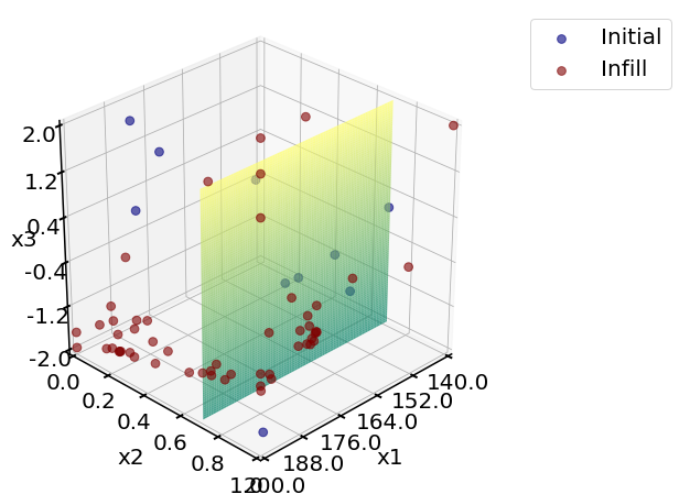
We would like to see how sampling points scattered in the 3D space. A 2D slices of the 3D space is visualized below at a fixed x value .

#%% plots
# Check the sampling points
# Final lhc Sampling
x2_fixed_real = 0.7 # fixed x2 value
x_indices = [0, 2] # 0-indexing, for x1 and x3
print('LHC sampling points')
plotting.sampling_3d_exp(Exp_lhc,
                         slice_axis = 'y',
                         slice_value_real = x2_fixed_real)

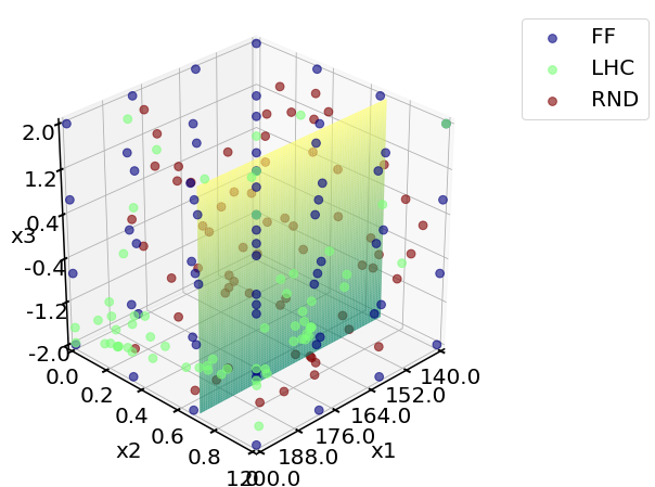
# Compare 3 sampling plans
print('Comparing 3 plans: ')
plotting.sampling_3d([Exp_ff.X, Exp_lhc.X, Exp_rnd.X],
                     X_ranges = X_ranges,
                     design_names = ['FF', 'LHC', 'RND'],
                     slice_axis = 'y',
                     slice_value_real = x2_fixed_real)

LHC sampling points

Comparing 3 plans:

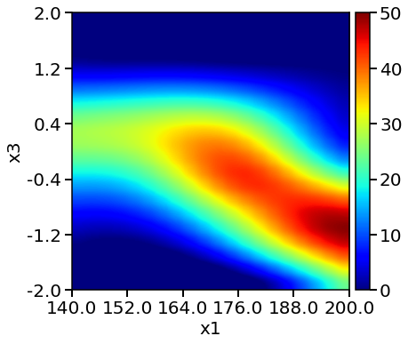
By fixing the value of pH (x2), we can plot the 2D reponse surfaces by varying T (x1) and tf (x3). It takes a long time to get the reponses from the objective function.

To create a heatmap, we generate mesh_size (by default = 41, here we set it as 20) test points along one dimension. For a 2D mesh, 20 by 20, i.e. 400 times of evaluation is needed. The following code indicates that evaluting the GP surrogate model is much faster than calling the objective function.

# Reponse heatmaps
# Set X_test mesh size
mesh_size = 20
n_test = mesh_size**2

# Objective function heatmap
# (this takes a long time)
print('Objective function heatmap: ')
start_time = time.time()
plotting.objective_heatmap(objective_func,
                          X_ranges,
                          Y_real_range = Y_plot_range,
                          x_indices = x_indices,
                          fixed_values_real = x2_fixed_real,
                          mesh_size = mesh_size)
end_time = time.time()
print('Evaluation of objective function {} times takes {:.2f} min\n'.format(n_test, (end_time-start_time)/60))


# full factorial heatmap
print('Full factorial model heatmap: ')
start_time = time.time()
plotting.response_heatmap_exp(Exp_ff,
                              Y_real_range = Y_plot_range,
                              x_indices = x_indices,
                              fixed_values_real = x2_fixed_real,
                              mesh_size = mesh_size)
end_time = time.time()
print('Evaluation of FF GP model {} times takes {:.2f} min\n'.format(n_test, (end_time-start_time)/60))


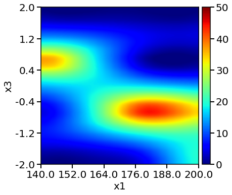
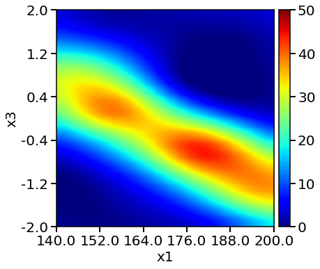
# LHC heatmap
print('LHC model heatmap: ')
start_time = time.time()
plotting.response_heatmap_exp(Exp_lhc,
                              Y_real_range = Y_plot_range,
                              x_indices = x_indices,
                              fixed_values_real = x2_fixed_real,
                              mesh_size = mesh_size)
end_time = time.time()
print('Evaluation of LHC GP model {} times takes {:.2f} min\n'.format(n_test, (end_time-start_time)/60))


# random sampling heatmap
print('RND model heatmap: ')
start_time = time.time()
plotting.response_heatmap_exp(Exp_rnd,
                              Y_real_range = Y_plot_range,
                              x_indices = x_indices,
                              fixed_values_real = x2_fixed_real,
                              mesh_size = mesh_size)
end_time = time.time()
print('Evaluation of RND GP model {} times takes {:.2f} min\n'.format(n_test, (end_time-start_time)/60))

Objective function heatmap:

C:\Users\yifan\Anaconda3\envs\torch\lib\site-packages\scipy\integrate\_ode.py:1182: UserWarning: dopri5: larger nsteps is needed
  self.messages.get(istate, unexpected_istate_msg)))

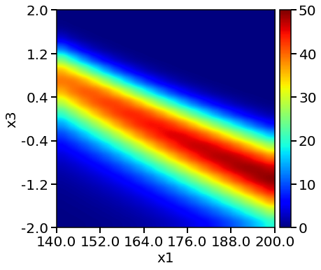
Evaluation of objective function 400 times takes 0.14 min

Full factorial model heatmap:

Evaluation of FF GP model 400 times takes 0.00 min

LHC model heatmap:

Evaluation of LHC GP model 400 times takes 0.00 min

RND model heatmap:

Evaluation of RND GP model 400 times takes 0.00 min

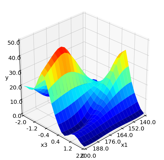
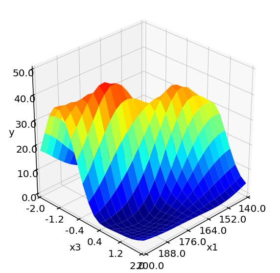
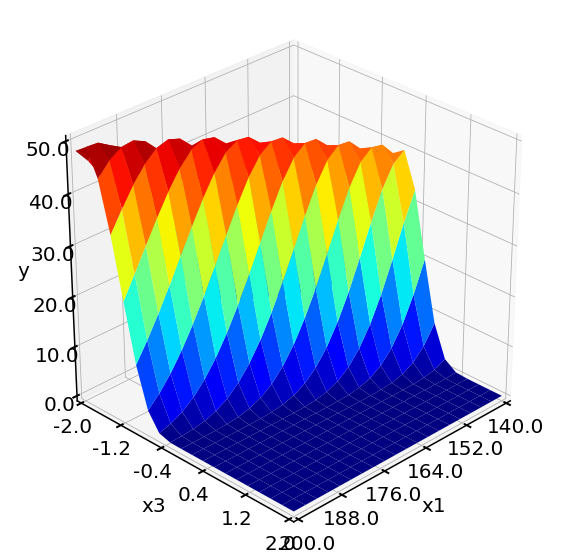
The rates can also be plotted as response surfaces in 3D.

# Suface plots
# Objective function surface plot
#(this takes a long time)
print('Objective function surface: ')
start_time = time.time()
plotting.objective_surface(objective_func,
                          X_ranges,
                          Y_real_range = Y_plot_range,
                          x_indices = x_indices,
                          fixed_values_real = x2_fixed_real,
                          mesh_size = mesh_size)
end_time = time.time()
print('Evaluation of objective function {} times takes {:.2f} min\n'.format(n_test, (end_time-start_time)/60))

# full fatorial surface plot
print('LHC model surface: ')
start_time = time.time()
plotting.response_surface_exp(Exp_ff,
                              Y_real_range = Y_plot_range,
                              x_indices = x_indices,
                              fixed_values_real = x2_fixed_real,
                              mesh_size = mesh_size)
end_time = time.time()
print('Evaluation of FF GP model {} times takes {:.2f} min\n'.format(n_test, (end_time-start_time)/60))


# LHC surface plot
print('Full fatorial model surface: ')
start_time = time.time()
plotting.response_surface_exp(Exp_lhc,
                              Y_real_range = Y_plot_range,
                              x_indices = x_indices,
                              fixed_values_real = x2_fixed_real,
                              mesh_size = mesh_size)
end_time = time.time()
print('Evaluation of LHC GP model {} times takes {:.2f} min\n'.format(n_test, (end_time-start_time)/60))


# random sampling surface plot
print('RND model surface: ')
start_time = time.time()
plotting.response_surface_exp(Exp_rnd,
                              Y_real_range = Y_plot_range,
                              x_indices = x_indices,
                              fixed_values_real = x2_fixed_real,
                              mesh_size = mesh_size)
end_time = time.time()
print('Evaluation of RND GP model {} times takes {:.2f} min\n'.format(n_test, (end_time-start_time)/60))

Objective function surface:

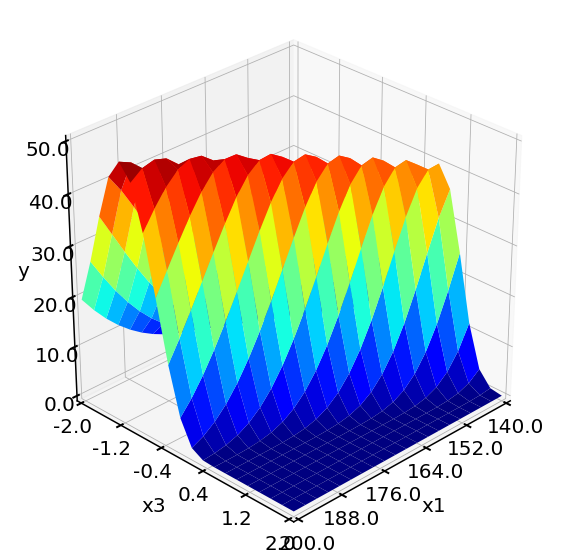
Evaluation of objective function 400 times takes 0.14 min

LHC model surface:

Evaluation of FF GP model 400 times takes 0.00 min

Full fatorial model surface:

Evaluation of LHC GP model 400 times takes 0.00 min

RND model surface:

Evaluation of RND GP model 400 times takes 0.00 min

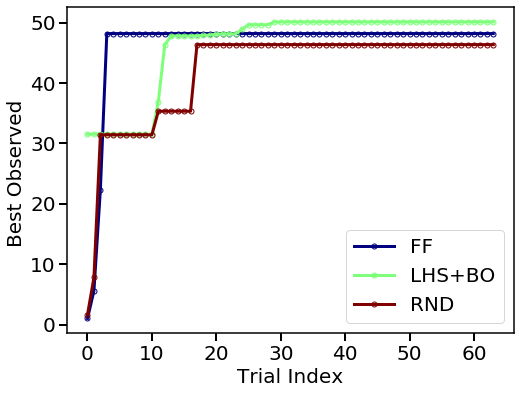
7. Export the optimum

Compare two plans in terms optimum discovered in each trial.

plotting.opt_per_trial([Exp_ff.Y_real, Exp_lhc.Y_real, Exp_rnd.Y_real],
                       design_names = ['FF', 'LHS+BO', 'RND'])

Obtain the optimum from each method.

# full factorial optimum
y_opt_ff, X_opt_ff, index_opt_ff = Exp_ff.get_optim()
data_opt_ff = io.np_to_dataframe([X_opt_ff, y_opt_ff], var_names)

print('From full factorial design, ')
display(data_opt_ff)


# lhc optimum
y_opt_lhc, X_opt_lhc, index_opt_lhc = Exp_lhc.get_optim()
data_opt_lhc = io.np_to_dataframe([X_opt_lhc, y_opt_lhc], var_names)

print('From LHS + Bayesian Optimization, ')
display(data_opt_lhc)


# random sampling optimum
y_opt_rnd, X_opt_rnd, index_opt_rnd = Exp_rnd.get_optim()
data_opt_rnd = io.np_to_dataframe([X_opt_rnd, y_opt_rnd], var_names)

print('From random sampling, ')
display(data_opt_rnd)

From full factorial design,

	T ($\rm ^{o}C $)	pH	$\rm log_{10}(tf_{min})$	Yield %
0	200.0	0.0	-2.0	48.179909

From LHS + Bayesian Optimization,

	T ($\rm ^{o}C $)	pH	$\rm log_{10}(tf_{min})$	Yield %
0	200.0	0.247871	-1.595599	50.101672

From random sampling,

	T ($\rm ^{o}C $)	pH	$\rm log_{10}(tf_{min})$	Yield %
0	180.730132	0.211628	-0.937813	46.353722

From above plots, we see the response surface produced by LHC + Bayesian Optimization is more accurate and resembles the one from the objective function. The method also locates a higher yield value compared to designs. We can conclude that LHC + Bayesian Optimization is efficient in locating the optimum and produce accurate surrogate models at affordable computational cost.

References:

1. Desir, P.; Saha, B.; Vlachos, D. G. Energy Environ. Sci. 2019.

2. Swift, T. D.; Bagia, C.; Choudhary, V.; Peklaris, G.; Nikolakis, V.; Vlachos, D. G. ACS Catal. 2014, 4 (1), 259–267

3. The PFR model can be found on GitHub: https://github.com/VlachosGroup/Fructose-HMF-Model

Thumbnail of this notebook