Example 1 - Simple 1d nonlinear function

In this example, we will show how to train a Gaussian Process (GP) surrogate model for a nonlinear function and locate its optimum via Bayesian Optimization. The objective function has an analytical form of

\[y = (6x-2)^2 sin(12x-4)\]

where x is the independent variable (input parameter) and y is the dependent variable (output response or target). The goal is locate the x value where y is optimized (minimized in this case).

The details of this example is summarized in the table below:

Key Item	Description
Goal	Minimization
Objective function	Simple nonlinear
Input (X) dimension	1
Output (Y) dimension	1
Analytical form available?	Yes
Acqucision function	Expected improvement (EI)
Initial Sampling	Grid search

Next, we will go through each step in Bayesian Optimization.

1. Import nextorch and other packages

import numpy as np
from nextorch import plotting, bo

2. Define the objective function and the design space

We use a Python function object as the objective function objective_func. The range of the input X_ranges is between 0 and 1, i.e., in a unit scale.

def simple_1d(X):
    """1D function y = (6x-2)^2 * sin(12x-4)

    Parameters
    ----------
    X : numpy array or a list
        1D independent variable

    Returns
    -------
    y: numpy array
        1D dependent variable
    """
    try:
        X.shape[1]
    except:
        X = np.array(X)
    if len(X.shape)<2:
        X = np.array([X])

    y = np.array([],dtype=float)

    for i in range(X.shape[0]):
        ynew = (X[i]*6-2)**2*np.sin((X[i]*6-2)*2)
        y = np.append(y, ynew)
    y = y.reshape(X.shape)

    return y

objective_func = simple_1d

3. Define the initial sampling plan

The initial sampling plan X_init can be a Design of Experiment (DOE), random sampling or grid search. In this example, since the input dimension is only 1, we can just do a grid search for x with a 0.25 interval.

The initial reponse Y_init is computed from the objective function.

# Create a grid with a 0.25 interval
X_init = np.array([[0, 0.25, 0.5, 0.75]]).T

# X_range is [0, 1], therefore we can get the reponse directly
# from the objective function
# Get the initial responses
Y_init = objective_func(X_init)
# Equavalent to
# Y_init = bo.eval_objective_func(X_init, X_ranges = [0,1], objective_func)

4. Initialize an Experiment object

The Experiment object is the core class in nextorch.

It consists of a Gaussian Process (GP) model Exp.model trained by the input data and an acquisition function acq_func which provides the next point to sample.

Some progress status will be printed out every time when we train a GP model.

# Initialize an Experiment object Exp
# Set its name, the files will be saved under the folder with the same name
Exp = bo.Experiment('simple_1d')
# Import the initial data
# Set unit_flag to true since the X is in a unit scale
Exp.input_data(X_init, Y_init, unit_flag = True)
# Set the optimization specifications
# Here we set the objective function, minimization as the goal
Exp.set_optim_specs(objective_func = objective_func, maximize = False)

Iter 10/100: 3.3208022117614746
Iter 20/100: 3.1972315311431885
Iter 30/100: 3.1579580307006836

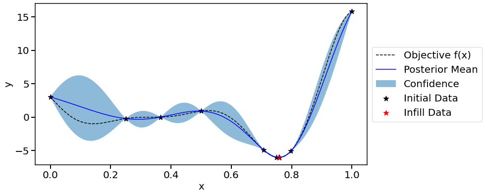
5. Run trials

We define one iteration of the experiment as a trial.

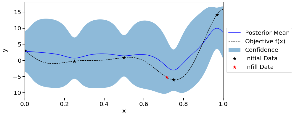
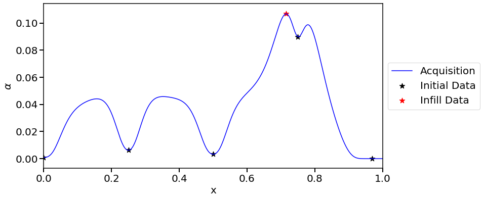
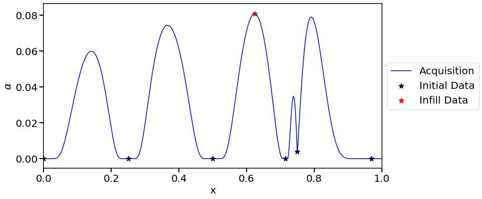
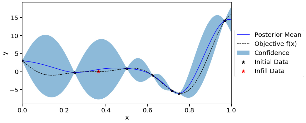
First, the next point(s) X_new_real to be run are suggested by the acquisition function. Next, the reponse at this point Y_new_real is computed from the objective function. We generate one point per trial in this experiment.

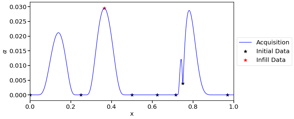
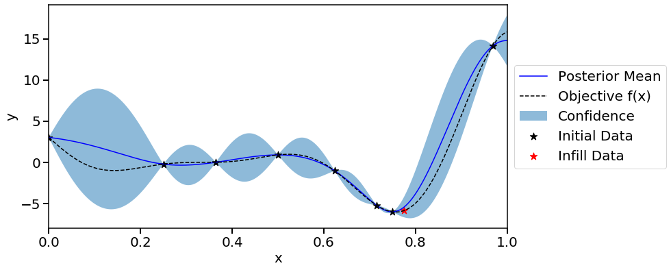
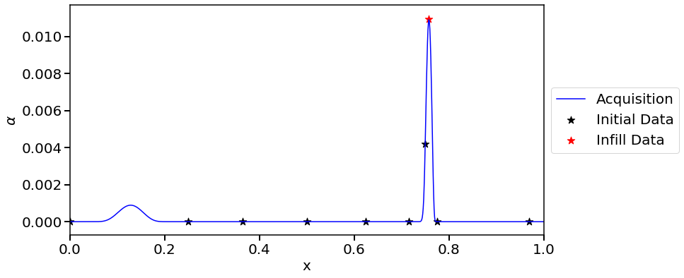
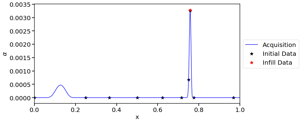
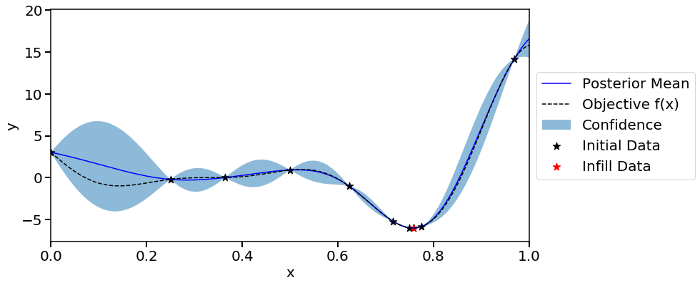
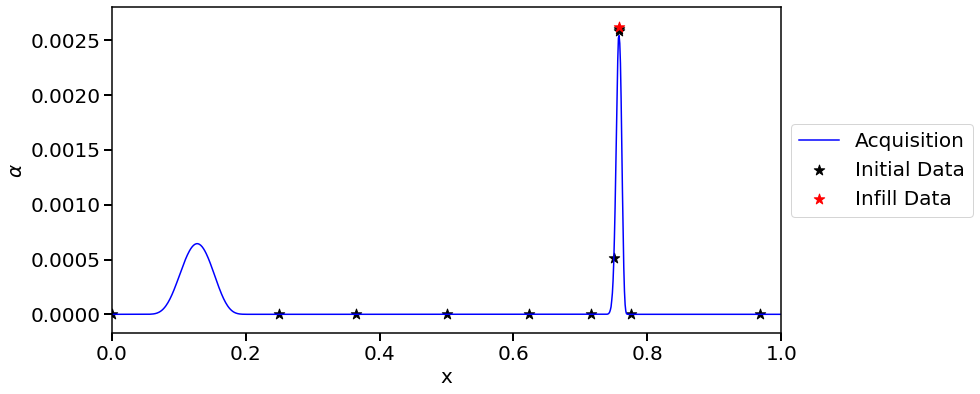
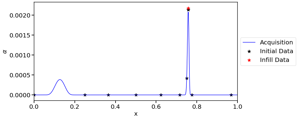
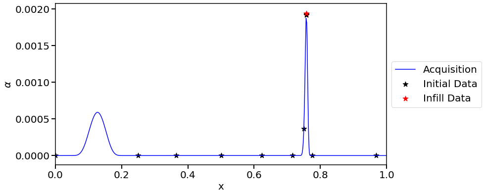
To plot the objective function and acquisition function value versus X, we create a set of mesh test points in the given range. The number of mesh points can be controlled by mesh_size parameter (here we use 1000). This process is repeated until the a stopping criteria is met.

The acquisition function Expected Improvement (EI) balances between exploitation and exploration. Generally, it is a good one to try first.

# Set a flag for saving png figures
save_fig_flag = False

# Set the number of iterations
n_trials = 10

# Optimization loop
for i in range(n_trials):
    # Generate the next experiment point
    # X_new is in a unit scale
    # X_new_real is in a real scale defined in X_ranges
    # Select EI as the acquisition function
    X_new, X_new_real, acq_func = Exp.generate_next_point(acq_func_name = 'EI')
    # Get the reponse at this point
    Y_new_real = objective_func(X_new_real)

    # Plot the objective functions, and acqucision function
    print('Iteration {}, objective function'.format(i+1))
    plotting.response_1d_exp(Exp,  X_new = X_new, mesh_size = 1000, plot_real = True, save_fig = save_fig_flag)
    print('Iteration {}, acquisition function'.format(i+1))
    plotting.acq_func_1d_exp(Exp, X_new = X_new, mesh_size = 1000, save_fig = save_fig_flag)

    # Input X and Y of the next point into Exp object
    # Retrain the model
    Exp.run_trial(X_new, X_new_real, Y_new_real)

Iteration 1, objective function

Iteration 1, acquisition function

Iter 10/100: 3.7735233306884766
Iter 20/100: 3.4933114051818848
Iter 30/100: 3.4236323833465576
Iter 40/100: 3.404162883758545
Iter 50/100: 3.3939692974090576
Iter 60/100: 3.388427734375
Iter 70/100: 3.3859429359436035
Iter 80/100: 3.3844447135925293
Iter 90/100: 3.3833441734313965
Iter 100/100: 3.3825888633728027
Iteration 2, objective function

Iteration 2, acquisition function

Iter 10/100: 3.0622379779815674
Iter 20/100: 3.0250864028930664
Iter 30/100: 2.97308087348938
Iteration 3, objective function

Iteration 3, acquisition function

Iteration 4, objective function

Iteration 4, acquisition function

Iteration 5, objective function

Iteration 5, acquisition function

Iter 10/100: 2.152087926864624
Iter 20/100: 2.14461612701416
Iter 30/100: 2.1397790908813477
Iter 40/100: 2.136268377304077
Iter 50/100: 2.133976936340332
Iter 60/100: 2.1323108673095703
Iter 70/100: 2.1310884952545166
Iter 80/100: 2.1301541328430176
Iter 90/100: 2.1294312477111816
Iter 100/100: 2.128840446472168
Iteration 6, objective function

Iteration 6, acquisition function

Iteration 7, objective function

Iteration 7, acquisition function

Iteration 8, objective function

Iteration 8, acquisition function

Iteration 9, objective function

Iteration 9, acquisition function

Iteration 10, objective function

Iteration 10, acquisition function

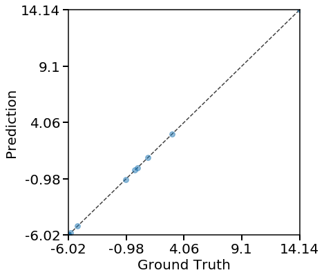
6. Validate the final model

We can get the optimum value from the Experiment object and validate the GP model predictions on the training data. The parity plots below show that the GP model agrees well with objective function values.

# Obtain the optimum
y_opt, X_opt, index_opt = Exp.get_optim()
print('The best reponse is Y = {} at X = {}'.format(y_opt, X_opt))

# Make a parity plot comparing model predictions versus ground truth values
plotting.parity_exp(Exp, save_fig = save_fig_flag)
# Make a parity plot with the confidence intervals on the predictions
plotting.parity_with_ci_exp(Exp, save_fig = save_fig_flag)

The best reponse is Y = -6.02073996139919 at X = [0.75726205]

Thumbnail of this notebook