Example 2 - Sin(x) 1d function¶

In this example, we will show how to locate the maximum of a simple 1d function via Bayesian Optimization. The objective function has an analytical form of

\[y = sin(x)\]

where x is the independent variable (input parameter) and y is the dependent variable (output response or target). The goal is locate the x value where y is optimized (maximized in this case).

The details of this example is summarized in the table below:

Key Item	Description
Goal	Maximization
Objective function	sin(x)
Input (X) dimension	1
Output (Y) dimension	1
Analytical form available?	Yes
Acqucision function	Expected improvement (EI)
Initial Sampling	Random

Next, we will go through each step in Bayesian Optimization.

1. Import `nextorch` and other packages¶

[1]:

import numpy as np
from nextorch import plotting, bo, doe, utils

2. Define the objective function and the design space¶

We use a Python lambda function as the objective function objective_func.

The range of the input X_ranges is between 0 and $2 \pi$.

[2]:

# Objective function
objective_func = lambda x: np.sin(x)

# Set the ranges
X_range = [0, np.pi*2]

3. Define the initial sampling plan¶

We choose 4 random points as the initial sampling plan X_init.

Note that X_init generated from doe methods are always in unit scales. If we want the sampling plan in real scales, we should use utils.inverse_unitscale_X(X_init, X_range) to obtain X_init_real.

The initial reponse in a real scale Y_init_real is computed from the objective function.

[3]:

# Randomly choose some points
# Sampling X is in a unit scale in [0, 1]
X_init = doe.randomized_design(n_dim = 1, n_points = 4, seed = 0)
#or we can do np.random.rand(4,1)

# Get the initial responses
Y_init_real = bo.eval_objective_func(X_init, X_range, objective_func)

# X in a real scale can be obtained via
X_init_real = utils.inverse_unitscale_X(X_init, X_range)
# The reponse can also be obtained by
# Y_init_real = objective_func(X_init_real)

4. Initialize an `Experiment` object¶

An Experiment requires the following key components: - Name of the experiment, used for output folder name - Input independent variables X: X_init or X_init_real - List of X ranges: X_ranges - Output dependent variables Y: Y_init or Y_init_real

Optional: - unit_flag: True if the input X matrix is a unit scale, else False - objective_func: Used for test plotting - maximize: True if we look for maximum, else False for minimum

[4]:

#%% Initialize an Experiment object
# Set its name, the files will be saved under the folder with the same name
Exp = bo.Experiment('sin_1d')
# Import the initial data
Exp.input_data(X_init, Y_init_real, unit_flag = True, X_ranges = X_range)


# Set the optimization specifications
# here we set the objective function, minimization by default
Exp.set_optim_specs(objective_func = objective_func, maximize= True)

Iter 10/100: 3.3435423374176025
Iter 20/100: 3.210638999938965
Iter 30/100: 3.1058804988861084
Iter 40/100: 2.723320484161377

5. Run trials¶

We use the same setup in the optimization loop as Example 1.

[5]:

# Set a flag for saving png figures
save_fig_flag = False

# Set the number of iterations
n_trials = 10

# Optimization loop
for i in range(n_trials):
    # Generate the next experiment point
    # X_new is in a unit scale
    # X_new_real is in a real scale defined in X_ranges
    # Select EI as the acquisition function
    X_new, X_new_real, acq_func = Exp.generate_next_point(acq_func_name = 'EI')
    # Get the reponse at this point
    Y_new_real = objective_func(X_new_real)

    # Plot the objective functions, and acqucision function
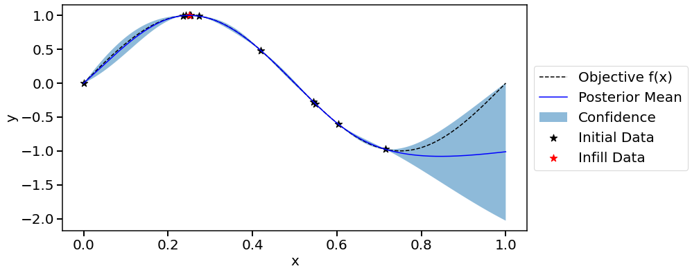
    print('Iteration {}, objective function'.format(i+1))
    plotting.response_1d_exp(Exp, X_new = X_new, mesh_size = 1000, plot_real = True, save_fig = save_fig_flag)
    print('Iteration {}, acquisition function'.format(i+1))
    plotting.acq_func_1d_exp(Exp, X_new = X_new, mesh_size = 1000, save_fig = save_fig_flag)

    # Input X and Y of the next point into Exp object
    # Retrain the model
    Exp.run_trial(X_new, X_new_real, Y_new_real)

Iteration 1, objective function

Iteration 1, acquisition function

Iter 10/100: 2.1364855766296387
Iter 20/100: 2.0631940364837646
Iter 30/100: 2.021515369415283
Iter 40/100: 1.993206262588501
Iter 50/100: 1.9716613292694092
Iter 60/100: 1.9547755718231201
Iter 70/100: 1.940943956375122
Iter 80/100: 1.929296851158142
Iter 90/100: 1.9191741943359375
Iter 100/100: 1.911110281944275
Iteration 2, objective function

Iteration 2, acquisition function

Iteration 3, objective function

Iteration 3, acquisition function

Iteration 4, objective function

Iteration 4, acquisition function

Iteration 5, objective function

Iteration 5, acquisition function

Iteration 6, objective function

Iteration 6, acquisition function

Iteration 7, objective function

Iteration 7, acquisition function

Iteration 8, objective function

Iteration 8, acquisition function

Iter 10/100: -0.20437514781951904
Iteration 9, objective function

Iteration 9, acquisition function

Iteration 10, objective function

Iteration 10, acquisition function

6. Validate the final model¶

Get the optimum value, locations, and plot the parity plot for training data.

For $sin(x)$ in $[0, 2\pi]$, the optimum should be $ y_{opt} = 1$ at $ x = \pi/2 $. We see the algorithm is able to place a point near the optimum region in iteration 2.

[6]:

# Obtain the optimum
y_opt, X_opt, index_opt = Exp.get_optim()
print('The best reponse is Y = {} at X = {}'.format(y_opt, X_opt))

# Make a parity plot comparing model predictions versus ground truth values
plotting.parity_exp(Exp, save_fig = save_fig_flag)
# Make a parity plot with the confidence intervals on the predictions
plotting.parity_with_ci_exp(Exp, save_fig = save_fig_flag)

The best reponse is Y = 0.9999998195370433 at X = [1.56981456]

Thumbnail of this notebook