Example 13 - Using AX for plug flow reactor yield optimization
In this notebook, we will demonstrate the syntax of Ax. Both Ax and NEXTorch are Python wrappers around BoTorch for Bayesian Optimization. By comparing to Example 5, the reader can see the differences in the synatx and designs of two software. We will use the loop and developer API for Ax, which corresponds to automatic and human-in-the-loop optimization.
From Example 5, the optimal value of the yield obtained by NEXTorhc is around 50.1%. We can see Ax reach a similar value.
Note: this notebook requires ax to be install first. See instructions on the Ax documentation page.
1. Import Ax and other packages
[12]:
import numpy as np
import os, sys
from IPython.display import display
import pprint
pp = pprint.PrettyPrinter(indent=4)

# ax functions from the loop API
from ax.service.managed_loop import optimize

# ax functions from the developer API
from ax import (
    Data,
    ParameterType,
    RangeParameter,
    SearchSpace,
    SimpleExperiment,
)
from ax.modelbridge.registry import Models

# ax visualization functions
from ax.plot.contour import plot_contour
from ax.plot.trace import optimization_trace_single_method
from ax.plot.slice import plot_slice
from ax.utils.notebook.plotting import render, init_notebook_plotting

init_notebook_plotting()
[INFO 09-25 21:45:45] ax.utils.notebook.plotting: Injecting Plotly library into cell. Do not overwrite or delete cell.
2. Define the objective function and the design space
[13]:
#%% Define the objective function
project_path = os.path.abspath(os.path.join(os.getcwd(), '..\..'))
sys.path.insert(0, project_path)

# Set the path for objective function
objective_path = os.path.join(project_path, 'examples', 'PFR')
sys.path.insert(0, objective_path)
from fructose_pfr_model_function import Reactor

#%% Define the design space
# Three input temperature C, pH, log10(residence time)
x_name_simple = ['T', 'pH', 'tf']
X_name_list = ['T', 'pH', r'$\rm log_{10}(tf_{min})$']
X_units = [r'$\rm ^{o}C $', '', '']

# Add the units
X_name_with_unit = []
for i, var in enumerate(X_name_list):
    if not X_units[i]  == '':
        var = var + ' ('+ X_units[i] + ')'
    X_name_with_unit.append(var)

# One output
Y_name_with_unit = 'Yield %'

# combine X and Y names
var_names = X_name_with_unit + [Y_name_with_unit]

# Set the operating range for each parameter
X_ranges =  [[140, 200], # Temperature ranges from 140-200 degree C
             [0, 1], # pH values ranges from 0-1
             [-2, 2]] # log10(residence time) ranges from -2-2

# Set the reponse range
Y_plot_range = [0, 50]

# Get the information of the design space
n_dim = len(X_name_list) # the dimension of inputs
n_objective = 1 # the dimension of outputs

# known optimal value from Example 5
y_known = 50.1

# Objective function
def objective_function(
    X_real, # dict of parameter names to values of those parameters
    weight=None, # optional weight argument
):
    # given a dict of parameter , compute a value for each metric
    x1 = X_real[x_name_simple[0]]
    x2 = X_real[x_name_simple[1]]
    x3 = X_real[x_name_simple[2]]

    Conditions = {'T_degC (C)': x1, 'pH': x2, 'tf (min)' : 10**x3}
    yi, _ = Reactor(**Conditions) # only keep the first output

    # a dictionary of objective names to tuples of mean and standard error for those objectives
    # the initial standard error is assume to be 0
    return {Y_name_with_unit: (yi, 0)}
3. Automatic optimization using the loop API
This is a lightweight API to use Ax for optimization. The initial sampling plan (usually Sobol sampling), acquisition function, and number of sampling points per trial are already fixed. The disadvantage is that it is often hard to customize the optimization loop.
[14]:
# set the total number of sampling points
n_total = 64
# optimization function main body
best_parameters_1, values_1, experiment_1, model_1 = optimize(
    parameters=[
        {
            "name": x_name_simple[0],
            "type": "range",
            "bounds": X_ranges[0],
            "value_type": "float",  # Optional, defaults to inference from type of "bounds".
            "log_scale": False,  # Optional, defaults to False.
        },
        {
            "name": x_name_simple[1],
            "type": "range",
            "bounds": X_ranges[1],
            "value_type": "float",
            "log_scale": False,
        },
        {
            "name": x_name_simple[2],
            "type": "range",
            "bounds": X_ranges[2],
            "value_type": "float",
            "log_scale": False,
        },
    ],
    experiment_name="PFR",
    objective_name=Y_name_with_unit,
    evaluation_function=objective_function,
    minimize=False,
    total_trials=n_total,
    arms_per_trial=1,
)

# the values of the best parameter
print('Optimal parameters:')
pp.pprint(best_parameters_1)

# the optimal objective value
print('Optimal objective value:')
pp.pprint(values_1)
[INFO 09-25 21:45:45] ax.modelbridge.dispatch_utils: Using GPEI (Bayesian optimization) since there are more continuous parameters than there are categories for the unordered categorical parameters.
[INFO 09-25 21:45:45] ax.modelbridge.dispatch_utils: Using Bayesian Optimization generation strategy: GenerationStrategy(name='Sobol+GPEI', steps=[Sobol for 5 trials, GPEI for subsequent trials]). Iterations after 5 will take longer to generate due to  model-fitting.
[INFO 09-25 21:45:45] ax.service.managed_loop: Started full optimization with 64 steps.
[INFO 09-25 21:45:45] ax.service.managed_loop: Running optimization trial 1...
[INFO 09-25 21:45:45] ax.service.managed_loop: Running optimization trial 2...
[INFO 09-25 21:45:45] ax.service.managed_loop: Running optimization trial 3...
[INFO 09-25 21:45:45] ax.service.managed_loop: Running optimization trial 4...
[INFO 09-25 21:45:46] ax.service.managed_loop: Running optimization trial 5...
[INFO 09-25 21:45:46] ax.service.managed_loop: Running optimization trial 6...
[INFO 09-25 21:45:46] ax.service.managed_loop: Running optimization trial 7...
[INFO 09-25 21:45:47] ax.service.managed_loop: Running optimization trial 8...
[INFO 09-25 21:45:47] ax.service.managed_loop: Running optimization trial 9...
[INFO 09-25 21:45:48] ax.service.managed_loop: Running optimization trial 10...
[INFO 09-25 21:45:49] ax.service.managed_loop: Running optimization trial 11...
[INFO 09-25 21:45:50] ax.service.managed_loop: Running optimization trial 12...
[INFO 09-25 21:45:51] ax.service.managed_loop: Running optimization trial 13...
[INFO 09-25 21:45:51] ax.service.managed_loop: Running optimization trial 14...
[INFO 09-25 21:45:52] ax.service.managed_loop: Running optimization trial 15...
[INFO 09-25 21:45:53] ax.service.managed_loop: Running optimization trial 16...
[INFO 09-25 21:45:54] ax.service.managed_loop: Running optimization trial 17...
[INFO 09-25 21:45:55] ax.service.managed_loop: Running optimization trial 18...
[INFO 09-25 21:45:56] ax.service.managed_loop: Running optimization trial 19...
[INFO 09-25 21:45:57] ax.service.managed_loop: Running optimization trial 20...
[INFO 09-25 21:45:57] ax.service.managed_loop: Running optimization trial 21...
[INFO 09-25 21:45:58] ax.service.managed_loop: Running optimization trial 22...
[INFO 09-25 21:46:00] ax.service.managed_loop: Running optimization trial 23...
[INFO 09-25 21:46:02] ax.service.managed_loop: Running optimization trial 24...
[INFO 09-25 21:46:02] ax.service.managed_loop: Running optimization trial 25...
[INFO 09-25 21:46:03] ax.service.managed_loop: Running optimization trial 26...
[INFO 09-25 21:46:04] ax.service.managed_loop: Running optimization trial 27...
[INFO 09-25 21:46:05] ax.service.managed_loop: Running optimization trial 28...
[INFO 09-25 21:46:06] ax.service.managed_loop: Running optimization trial 29...
C:\Users\yifan\Anaconda3\envs\torch\lib\site-packages\scipy\integrate\_ode.py:1182: UserWarning:

dopri5: larger nsteps is needed

[INFO 09-25 21:46:07] ax.service.managed_loop: Running optimization trial 30...
[INFO 09-25 21:46:08] ax.service.managed_loop: Running optimization trial 31...
[INFO 09-25 21:46:09] ax.service.managed_loop: Running optimization trial 32...
[INFO 09-25 21:46:10] ax.service.managed_loop: Running optimization trial 33...
[INFO 09-25 21:46:11] ax.service.managed_loop: Running optimization trial 34...
[INFO 09-25 21:46:12] ax.service.managed_loop: Running optimization trial 35...
[INFO 09-25 21:46:12] ax.service.managed_loop: Running optimization trial 36...
[INFO 09-25 21:46:14] ax.service.managed_loop: Running optimization trial 37...
[INFO 09-25 21:46:15] ax.service.managed_loop: Running optimization trial 38...
[INFO 09-25 21:46:16] ax.service.managed_loop: Running optimization trial 39...
[INFO 09-25 21:46:18] ax.service.managed_loop: Running optimization trial 40...
[INFO 09-25 21:46:22] ax.service.managed_loop: Running optimization trial 41...
[INFO 09-25 21:46:24] ax.service.managed_loop: Running optimization trial 42...
[INFO 09-25 21:46:26] ax.service.managed_loop: Running optimization trial 43...
[INFO 09-25 21:46:26] ax.service.managed_loop: Running optimization trial 44...
C:\Users\yifan\Anaconda3\envs\torch\lib\site-packages\scipy\integrate\_ode.py:1182: UserWarning:

dopri5: larger nsteps is needed

[INFO 09-25 21:46:27] ax.service.managed_loop: Running optimization trial 45...
[INFO 09-25 21:46:28] ax.service.managed_loop: Running optimization trial 46...
[INFO 09-25 21:46:29] ax.service.managed_loop: Running optimization trial 47...
[INFO 09-25 21:46:31] ax.service.managed_loop: Running optimization trial 48...
[INFO 09-25 21:46:32] ax.service.managed_loop: Running optimization trial 49...
[INFO 09-25 21:46:34] ax.service.managed_loop: Running optimization trial 50...
[INFO 09-25 21:46:34] ax.service.managed_loop: Running optimization trial 51...
[INFO 09-25 21:46:35] ax.service.managed_loop: Running optimization trial 52...
[INFO 09-25 21:46:36] ax.service.managed_loop: Running optimization trial 53...
[INFO 09-25 21:46:38] ax.service.managed_loop: Running optimization trial 54...
[INFO 09-25 21:46:40] ax.service.managed_loop: Running optimization trial 55...
[INFO 09-25 21:46:42] ax.service.managed_loop: Running optimization trial 56...
[INFO 09-25 21:46:43] ax.service.managed_loop: Running optimization trial 57...
[INFO 09-25 21:46:44] ax.service.managed_loop: Running optimization trial 58...
[INFO 09-25 21:46:46] ax.service.managed_loop: Running optimization trial 59...
[INFO 09-25 21:46:48] ax.service.managed_loop: Running optimization trial 60...
[INFO 09-25 21:46:50] ax.service.managed_loop: Running optimization trial 61...
[INFO 09-25 21:46:52] ax.service.managed_loop: Running optimization trial 62...
[INFO 09-25 21:46:54] ax.service.managed_loop: Running optimization trial 63...
[INFO 09-25 21:46:56] ax.service.managed_loop: Running optimization trial 64...
Optimal parameters:
{'T': 200.0, 'pH': 0.5126827382174883, 'tf': -1.3324093248882605}
Optimal objective value:
(   {'Yield %': 50.10119996393495},
    {'Yield %': {'Yield %': 2.6388860573819856e-05}})
Visualize the final model reponses
By fixing the value of pH (x2), we plot the 2D reponse surfaces by varying T (x1) and tf (x3).
[15]:
x2_fixed_real = 0.7 # fixed x2 value
x_indices = [0, 2] # 0-indexing, for x1 and x3

slice_values = {x_name_simple[1]: x2_fixed_real}
contour_plot = plot_contour(model=model_1,
                    param_x=x_name_simple[x_indices[0]],
                    param_y=x_name_simple[x_indices[1]],
                    metric_name=Y_name_with_unit,
                    slice_values=slice_values)
render(contour_plot)
Plot the optimum discovred in each trial.
[16]:
# collect the objective values from each trial
objectives_values_1 = np.array([[trial.objective_mean for trial in experiment_1.trials.values()]])

best_objective_plot = optimization_trace_single_method(
    y=np.maximum.accumulate(objectives_values_1, axis=1),
    optimum=y_known,
    title="Model performance vs. # of iterations",
    ylabel=Y_name_with_unit,
)
render(best_objective_plot)
4. Human-in-the-loop optimization with the developer API
The developer API allows customization of the optimization loop. To introduce human-in-the-loop optimization, we explicitly convert the sampling points predicted by the acquisition function to a pandas Dataframe (data_all). Next, experiments shall be performed at these parameter values (in data_next) and the objective values shall be collected. A new Dataframe (data_new) containing all previous points is then needed to be passed a GP model. We show that multiple points can be taken
at each trial.
Since the objective function is passed into the SimpleExperiment object at the beginning, the evalution of objective function is still wrapped under the hood. However, for the majority of laboratory experiments, the objective function is unknown a priori. We do not know the best way to construct an Experiment object with no objective function input, or how to export the next sampling points before objective function evalution. These are all important elements for the human-in-the-loop
design.
For NEXTorch syntax, readers can refer to Example 4. No objective function input is required for an Experiment object.
[17]:
n_init = 10 #initial experiments
n_samples_per_trial = 3 # number of sampling points per trial
n_trials = int((n_total-n_init)/n_samples_per_trial) #number of trials

# define the parameter space (or search space)
search_space = SearchSpace(
    parameters=[
        RangeParameter(
            name=x_name_i, parameter_type=ParameterType.FLOAT, lower=X_range_i[0], upper=X_range_i[1]
        )
        for x_name_i, X_range_i in zip(x_name_simple, X_ranges)
    ]
)

# initialize a SimpleExperiment object
experiment_2 = SimpleExperiment(
    name="PFR",
    search_space=search_space,
    evaluation_function=objective_function,
    objective_name=Y_name_with_unit,
    minimize=False,
)

# Define Initial Sobol sampling plan
print("Running Sobol initialization trials...")
sobol = Models.SOBOL(experiment_2.search_space)
for i in range(n_init):
    experiment_2.new_trial(generator_run=sobol.gen(1))

# Show the initial sampling points
print("The initial sampling data: ")
data_all = experiment_2.eval().df
display(data_all)
Running Sobol initialization trials...
The initial sampling data:
C:\Users\yifan\Anaconda3\envs\torch\lib\site-packages\scipy\integrate\_ode.py:1182: UserWarning:

dopri5: larger nsteps is needed
| arm_name | metric_name | mean | sem | trial_index | |
|---|---|---|---|---|---|
| 0 | 0_0 | Yield % | 7.952644e+00 | 0.0 | 0 |
| 1 | 1_0 | Yield % | -5.432170e-11 | 0.0 | 1 |
| 2 | 2_0 | Yield % | 3.105702e+01 | 0.0 | 2 |
| 3 | 3_0 | Yield % | 4.790725e-02 | 0.0 | 3 |
| 4 | 4_0 | Yield % | 1.884997e+00 | 0.0 | 4 |
| 5 | 5_0 | Yield % | 4.747235e+01 | 0.0 | 5 |
| 6 | 6_0 | Yield % | 9.640585e+00 | 0.0 | 6 |
| 7 | 7_0 | Yield % | 5.101536e+00 | 0.0 | 7 |
| 8 | 8_0 | Yield % | 4.330709e+01 | 0.0 | 8 |
| 9 | 9_0 | Yield % | 2.424362e+01 | 0.0 | 9 |
[18]:
# Optimization loop main body
for i in range(n_trials):
    print(f"Running GP+EI optimization trial {i+1}/{n_trials}...")
    # Import the dataframe containing all previous point
    # Reinitialize GP+EI model at each step with the updated data
    data_new = Data(data_all)
    model_2 = Models.BOTORCH(experiment=experiment_2, data=data_new)
    experiment_2.new_batch_trial(generator_run=model_2.gen(n=3))

    # Export the next sampling points into a dataframe
    data_all = experiment_2.eval().df
    data_next = data_all[-n_samples_per_trial:]
    print(f"The new data points in iteration {i+1} are:")
    display(data_next)


print("Done!")
Running GP+EI optimization trial 1/18...
The new data points in iteration 1 are:
| arm_name | metric_name | mean | sem | trial_index | |
|---|---|---|---|---|---|
| 10 | 10_0 | Yield % | 41.298076 | 0.0 | 10 |
| 11 | 10_1 | Yield % | 46.843116 | 0.0 | 10 |
| 12 | 10_2 | Yield % | 47.403937 | 0.0 | 10 |
Running GP+EI optimization trial 2/18...
The new data points in iteration 2 are:
| arm_name | metric_name | mean | sem | trial_index | |
|---|---|---|---|---|---|
| 13 | 11_0 | Yield % | 47.058547 | 0.0 | 11 |
| 14 | 11_1 | Yield % | 43.302009 | 0.0 | 11 |
| 15 | 11_2 | Yield % | 38.391249 | 0.0 | 11 |
Running GP+EI optimization trial 3/18...
The new data points in iteration 3 are:
| arm_name | metric_name | mean | sem | trial_index | |
|---|---|---|---|---|---|
| 16 | 12_0 | Yield % | 44.782317 | 0.0 | 12 |
| 17 | 12_1 | Yield % | 46.967598 | 0.0 | 12 |
| 18 | 12_2 | Yield % | 45.833647 | 0.0 | 12 |
Running GP+EI optimization trial 4/18...
The new data points in iteration 4 are:
| arm_name | metric_name | mean | sem | trial_index | |
|---|---|---|---|---|---|
| 19 | 13_0 | Yield % | 47.867416 | 0.0 | 13 |
| 20 | 13_1 | Yield % | 48.093134 | 0.0 | 13 |
| 21 | 13_2 | Yield % | 45.756795 | 0.0 | 13 |
Running GP+EI optimization trial 5/18...
The new data points in iteration 5 are:
| arm_name | metric_name | mean | sem | trial_index | |
|---|---|---|---|---|---|
| 22 | 14_0 | Yield % | 47.481168 | 0.0 | 14 |
| 23 | 14_1 | Yield % | 49.071212 | 0.0 | 14 |
| 24 | 14_2 | Yield % | 49.291180 | 0.0 | 14 |
Running GP+EI optimization trial 6/18...
The new data points in iteration 6 are:
| arm_name | metric_name | mean | sem | trial_index | |
|---|---|---|---|---|---|
| 25 | 15_0 | Yield % | 47.982709 | 0.0 | 15 |
| 26 | 15_1 | Yield % | 49.012296 | 0.0 | 15 |
| 27 | 15_2 | Yield % | 20.783304 | 0.0 | 15 |
Running GP+EI optimization trial 7/18...
The new data points in iteration 7 are:
| arm_name | metric_name | mean | sem | trial_index | |
|---|---|---|---|---|---|
| 28 | 16_0 | Yield % | 49.037532 | 0.0 | 16 |
| 29 | 16_1 | Yield % | 49.942003 | 0.0 | 16 |
| 30 | 16_2 | Yield % | 48.650191 | 0.0 | 16 |
Running GP+EI optimization trial 8/18...
The new data points in iteration 8 are:
| arm_name | metric_name | mean | sem | trial_index | |
|---|---|---|---|---|---|
| 31 | 17_0 | Yield % | 48.310584 | 0.0 | 17 |
| 32 | 17_1 | Yield % | 44.241994 | 0.0 | 17 |
| 33 | 17_2 | Yield % | 35.070482 | 0.0 | 17 |
Running GP+EI optimization trial 9/18...
The new data points in iteration 9 are:
| arm_name | metric_name | mean | sem | trial_index | |
|---|---|---|---|---|---|
| 34 | 18_0 | Yield % | 44.510480 | 0.0 | 18 |
| 35 | 18_1 | Yield % | 49.309863 | 0.0 | 18 |
| 36 | 18_2 | Yield % | 49.531132 | 0.0 | 18 |
Running GP+EI optimization trial 10/18...
C:\Users\yifan\Anaconda3\envs\torch\lib\site-packages\gpytorch\utils\cholesky.py:44: NumericalWarning:

A not p.d., added jitter of 1.0e-08 to the diagonal

C:\Users\yifan\Anaconda3\envs\torch\lib\site-packages\gpytorch\utils\cholesky.py:44: NumericalWarning:

A not p.d., added jitter of 1.0e-08 to the diagonal
The new data points in iteration 10 are:
| arm_name | metric_name | mean | sem | trial_index | |
|---|---|---|---|---|---|
| 37 | 19_0 | Yield % | -4.297795e-11 | 0.0 | 19 |
| 38 | 19_1 | Yield % | 3.582672e+01 | 0.0 | 19 |
| 39 | 19_2 | Yield % | 4.144920e+01 | 0.0 | 19 |
Running GP+EI optimization trial 11/18...
The new data points in iteration 11 are:
| arm_name | metric_name | mean | sem | trial_index | |
|---|---|---|---|---|---|
| 40 | 20_0 | Yield % | 48.940496 | 0.0 | 20 |
| 41 | 20_1 | Yield % | 45.412358 | 0.0 | 20 |
| 42 | 20_2 | Yield % | 49.999238 | 0.0 | 20 |
Running GP+EI optimization trial 12/18...
The new data points in iteration 12 are:
| arm_name | metric_name | mean | sem | trial_index | |
|---|---|---|---|---|---|
| 43 | 21_0 | Yield % | 50.098608 | 0.0 | 21 |
| 44 | 21_1 | Yield % | 48.458128 | 0.0 | 21 |
| 45 | 21_2 | Yield % | 48.179908 | 0.0 | 21 |
Running GP+EI optimization trial 13/18...
C:\Users\yifan\Anaconda3\envs\torch\lib\site-packages\gpytorch\utils\cholesky.py:44: NumericalWarning:

A not p.d., added jitter of 1.0e-08 to the diagonal
The new data points in iteration 13 are:
C:\Users\yifan\Anaconda3\envs\torch\lib\site-packages\scipy\integrate\_ode.py:1182: UserWarning:

dopri5: larger nsteps is needed
| arm_name | metric_name | mean | sem | trial_index | |
|---|---|---|---|---|---|
| 46 | 22_0 | Yield % | 4.978738e+01 | 0.0 | 22 |
| 47 | 22_1 | Yield % | -5.399813e-11 | 0.0 | 22 |
| 48 | 22_2 | Yield % | 2.792262e+01 | 0.0 | 22 |
Running GP+EI optimization trial 14/18...
The new data points in iteration 14 are:
| arm_name | metric_name | mean | sem | trial_index | |
|---|---|---|---|---|---|
| 49 | 23_0 | Yield % | 49.960202 | 0.0 | 23 |
| 50 | 23_1 | Yield % | 50.092853 | 0.0 | 23 |
| 51 | 23_2 | Yield % | 48.490446 | 0.0 | 23 |
Running GP+EI optimization trial 15/18...
The new data points in iteration 15 are:
| arm_name | metric_name | mean | sem | trial_index | |
|---|---|---|---|---|---|
| 52 | 24_0 | Yield % | 49.938541 | 0.0 | 24 |
| 53 | 24_1 | Yield % | 49.631065 | 0.0 | 24 |
| 54 | 24_2 | Yield % | 50.055893 | 0.0 | 24 |
Running GP+EI optimization trial 16/18...
The new data points in iteration 16 are:
| arm_name | metric_name | mean | sem | trial_index | |
|---|---|---|---|---|---|
| 55 | 25_0 | Yield % | 1.069913 | 0.0 | 25 |
| 56 | 25_1 | Yield % | 49.932068 | 0.0 | 25 |
| 57 | 25_2 | Yield % | 10.203983 | 0.0 | 25 |
Running GP+EI optimization trial 17/18...
The new data points in iteration 17 are:
| arm_name | metric_name | mean | sem | trial_index | |
|---|---|---|---|---|---|
| 58 | 26_0 | Yield % | 50.095001 | 0.0 | 26 |
| 59 | 26_1 | Yield % | 49.129794 | 0.0 | 26 |
| 60 | 26_2 | Yield % | 47.987654 | 0.0 | 26 |
Running GP+EI optimization trial 18/18...
The new data points in iteration 18 are:
| arm_name | metric_name | mean | sem | trial_index | |
|---|---|---|---|---|---|
| 61 | 27_0 | Yield % | 50.093298 | 0.0 | 27 |
| 62 | 27_1 | Yield % | 27.434912 | 0.0 | 27 |
| 63 | 27_2 | Yield % | 49.155569 | 0.0 | 27 |
Done!
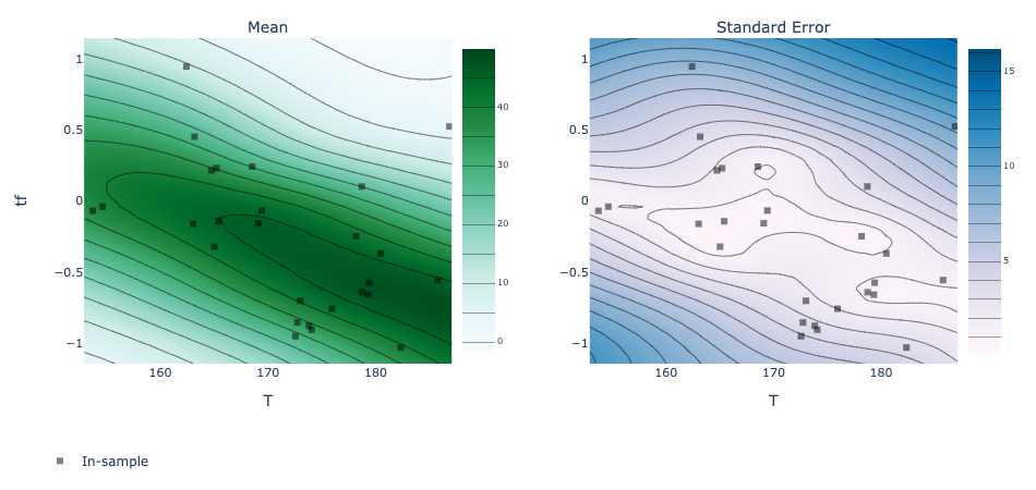
Visualize the final model reponses
By fixing the value of pH (x2), we plot the 2D reponse surfaces by varying T (x1) and tf (x3).
[19]:
x2_fixed_real = 0.7 # fixed x2 value
x_indices = [0, 2] # 0-indexing, for x1 and x3

slice_values = {x_name_simple[1]: x2_fixed_real}
contour_plot = plot_contour(model=model_2,
                    param_x=x_name_simple[x_indices[0]],
                    param_y=x_name_simple[x_indices[1]],
                    metric_name=Y_name_with_unit,
                    slice_values=slice_values)
render(contour_plot)
By fixing the value of T (x1) and pH (x2), we plot the 1D reponse by varying and tf (x3).
[20]:
# set the fixed parameter values
slice_values = { x_name_simple[0]: np.max(X_ranges[0]),
                x_name_simple[1]: x2_fixed_real}
print('Fixed parameter values:')

pp.pprint(slice_values)
render(plot_slice(model_2, x_name_simple[2], Y_name_with_unit, slice_values = slice_values))
Fixed parameter values:
{'T': 200, 'pH': 0.7}
Plot the optimum discovered in each trial.
[21]:
# collect the objective values from the final Dataframe
objective_values_2 = np.array([data_all['mean']])

best_objective_plot = optimization_trace_single_method(
    y=np.maximum.accumulate(objective_values_2, axis = 1),
    optimum=y_known,
    title="Model performance vs. # of iterations",
    ylabel=Y_name_with_unit,
)
render(best_objective_plot)
Thumbnail of this notebook